simmr: quick start guide

Andrew Parnell

2023-10-27

Step 1: install simmr

Use:

install.packages("simmr")

then

library(simmr)

Step 2: load in the data

Some geese isotope data is included with this package. Find where it is with:

system.file("extdata", "geese_data.xls", package = "simmr")

Load into R with:

library(readxl)
path <- system.file("extdata", "geese_data.xls", package = "simmr")
geese_data <- lapply(excel_sheets(path), read_excel, path = path)

If you want to see what the original Excel sheet looks like you can run system(paste('open',path)).

We can now separate out the data into parts

targets <- geese_data[[1]]
sources <- geese_data[[2]]
TEFs <- geese_data[[3]]
concdep <- geese_data[[4]]

Note that if you don’t have TEFs or concentration dependence you can set these all to the value 0 or just leave them blank in the step below.

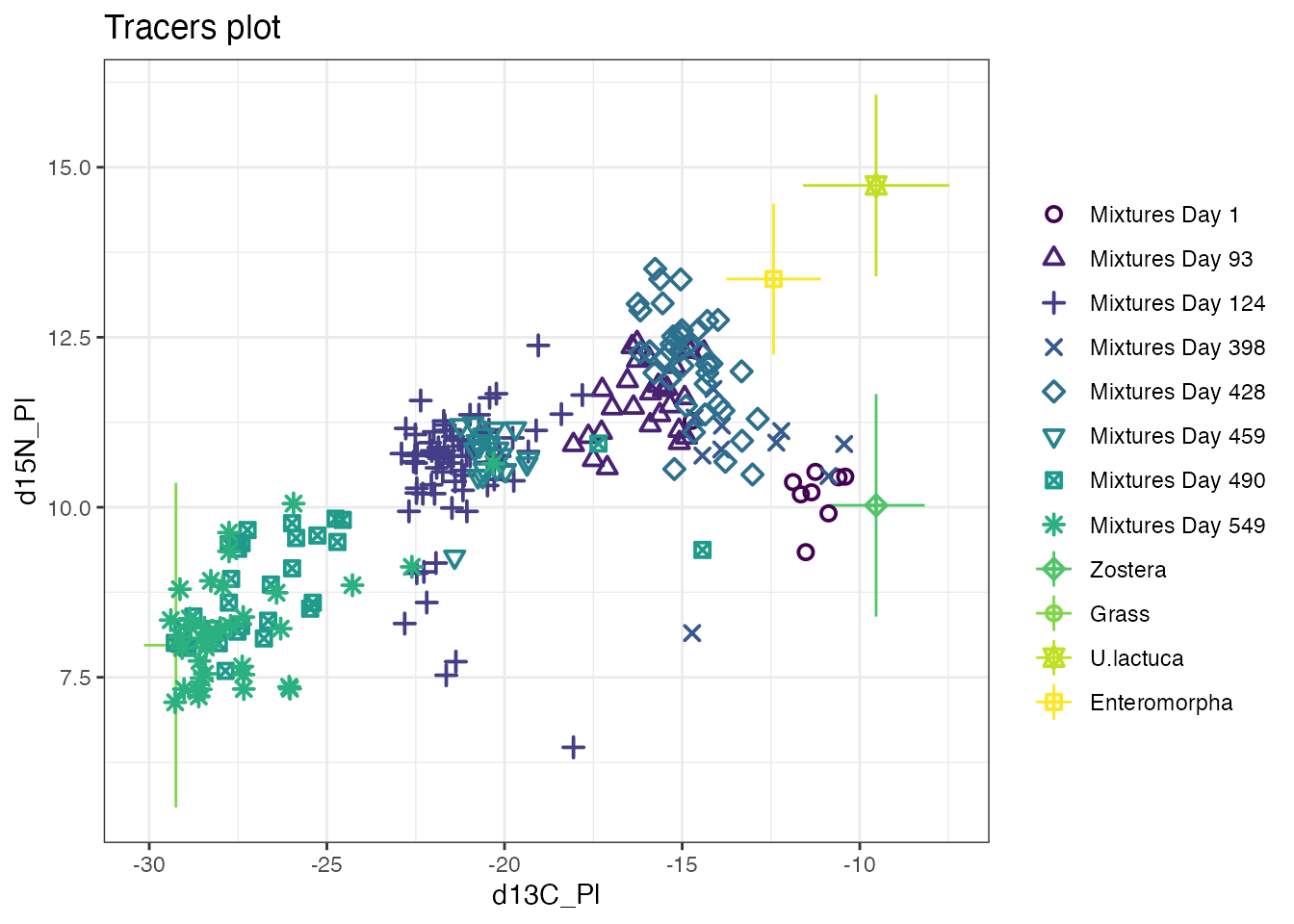
Step 3: load the data into simmr

geese_simmr <- simmr_load(
  mixtures = targets[, 1:2],
  source_names = sources$Sources,
  source_means = sources[, 2:3],
  source_sds = sources[, 4:5],
  correction_means = TEFs[, 2:3],
  correction_sds = TEFs[, 4:5],
  concentration_means = concdep[, 2:3],
  group = as.factor(paste("Day", targets$Time))
)

Step 4: plot the data

plot(geese_simmr, group = 1:8)

Step 5: run through simmr and check convergence

geese_simmr_out <- simmr_mcmc(geese_simmr)
summary(geese_simmr_out,
  type = "diagnostics",
  group = 1
)

Check that the model fitted well:

posterior_predictive(geese_simmr_out, group = 5)

## Compiling model graph
##    Resolving undeclared variables
##    Allocating nodes
## Graph information:
##    Observed stochastic nodes: 40
##    Unobserved stochastic nodes: 46
##    Total graph size: 198
## 
## Initializing model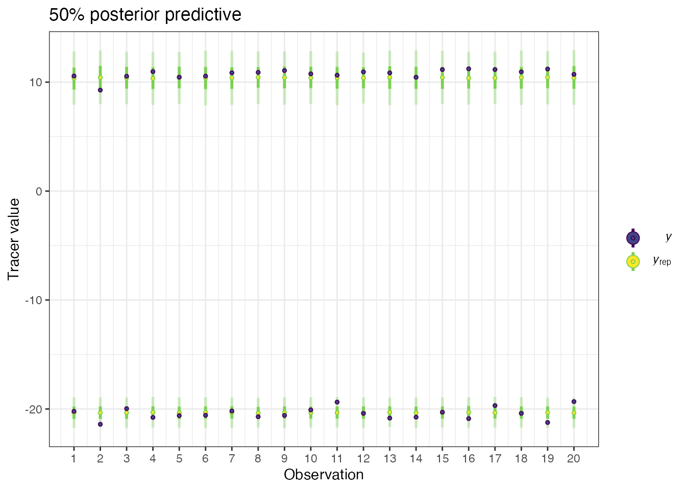

Step 6: look at the output

Look at the influence of the prior:

prior_viz(geese_simmr_out)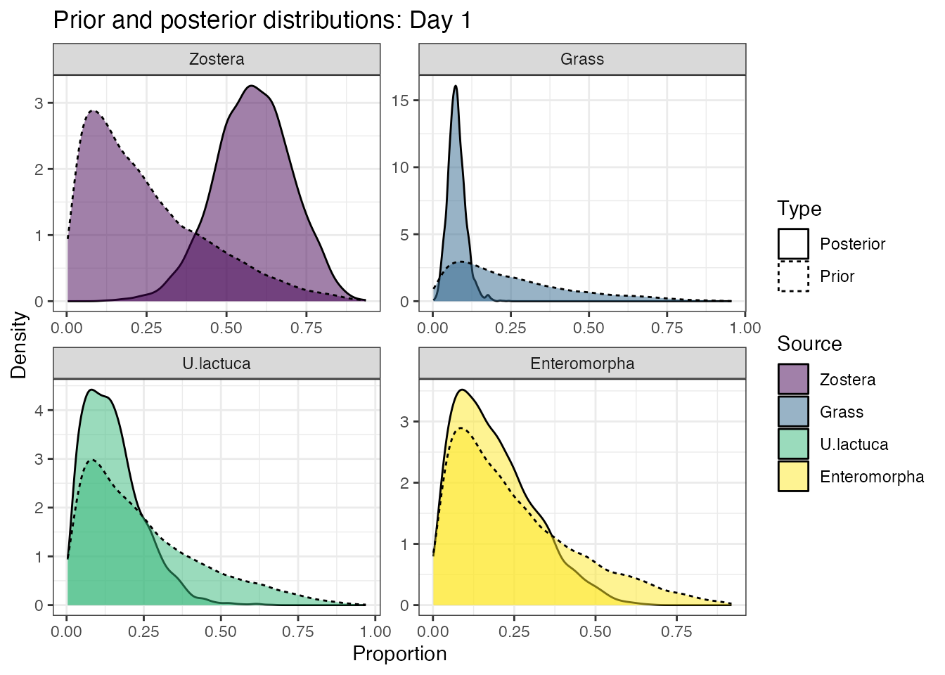

Look at the histogram of the dietary proportions:

plot(geese_simmr_out, type = "histogram")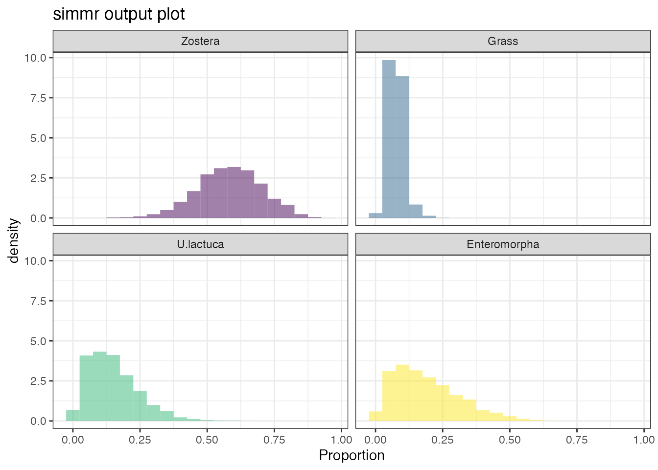

compare_groups(geese_simmr_out,
  groups = 1:4,
  source_name = "Enteromorpha"
)

## Most popular orderings are as follows:

##                                     Probability
## Day 428 > Day 124 > Day 398 > Day 1      0.2064
## Day 428 > Day 124 > Day 1 > Day 398      0.1711
## Day 428 > Day 398 > Day 124 > Day 1      0.1686
## Day 428 > Day 398 > Day 1 > Day 124      0.1031
## Day 428 > Day 1 > Day 124 > Day 398      0.0822
## Day 428 > Day 1 > Day 398 > Day 124      0.0706
## Day 398 > Day 428 > Day 124 > Day 1      0.0425
## Day 124 > Day 428 > Day 398 > Day 1      0.0389
## Day 124 > Day 428 > Day 1 > Day 398      0.0336
## Day 398 > Day 428 > Day 1 > Day 124      0.0206
## Day 398 > Day 124 > Day 428 > Day 1      0.0158
## Day 124 > Day 398 > Day 428 > Day 1      0.0117
## Day 1 > Day 428 > Day 124 > Day 398      0.0114
## Day 1 > Day 428 > Day 398 > Day 124      0.0067
## Day 398 > Day 1 > Day 428 > Day 124      0.0036
## Day 124 > Day 1 > Day 428 > Day 398      0.0033
## Day 1 > Day 124 > Day 428 > Day 398      0.0028
## Day 124 > Day 398 > Day 1 > Day 428      0.0019
## Day 124 > Day 1 > Day 398 > Day 428      0.0017
## Day 398 > Day 124 > Day 1 > Day 428      0.0017
## Day 398 > Day 1 > Day 124 > Day 428      0.0008
## Day 1 > Day 398 > Day 428 > Day 124      0.0006
## Day 1 > Day 124 > Day 398 > Day 428      0.0003
## Day 1 > Day 398 > Day 124 > Day 428      0.0003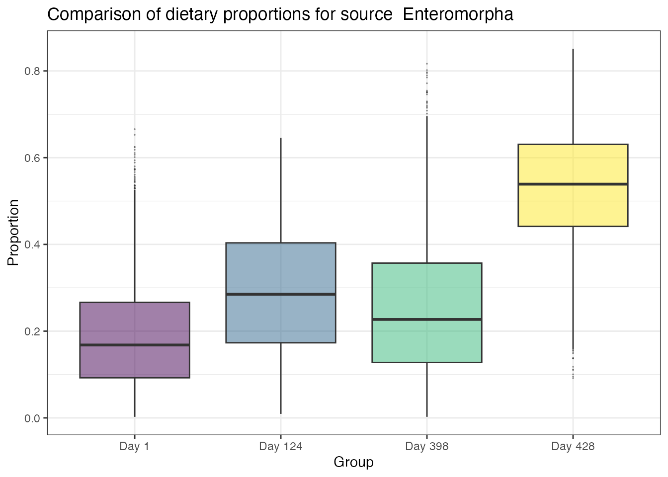

For the many more options available to run and analyse output, see the main vignette via vignette('simmr')