Plot the posterior predictive distribution for a simmr run

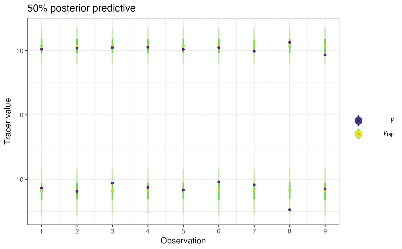
This function takes the output from simmr_mcmcand plots the posterior predictive distribution to enable visualisation of model fit. The simulated posterior predicted values are returned as part of the object and can be saved for external use

posterior_predictive(simmr_out, group = 1, prob = 0.5, plot_ppc = TRUE)

Arguments

simmr_out

A run of the simmr model from simmr_mcmc

group

Which group to run it for (currently only numeric rather than group names)

prob

The probability interval for the posterior predictives. The default is 0.5 (i.e. 50pc intervals)

plot_ppc

Whether to create a bayesplot of the posterior predictive or not.

Value

plot of posterior predictives and simulated values

Examples

# \donttest{
data(geese_data_day1)
simmr_1 <- with(
  geese_data_day1,
  simmr_load(
    mixtures = mixtures,
    source_names = source_names,
    source_means = source_means,
    source_sds = source_sds,
    correction_means = correction_means,
    correction_sds = correction_sds,
    concentration_means = concentration_means
  )
)

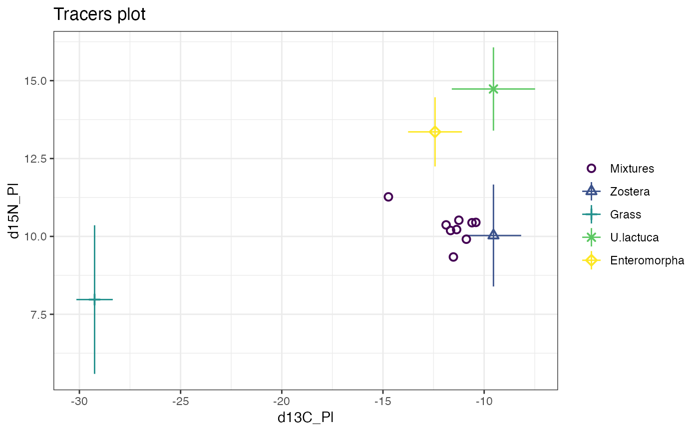
# Plot
plot(simmr_1)


# Print
simmr_1
#> This is a valid simmr input object with 
#> 9  observations, 
#> 2 tracers, and 
#> 4 sources.
#> The source names are: 
#> [1] "Zostera"      "Grass"        "U.lactuca"    "Enteromorpha"
#> .
#> The tracer names are: 
#> [1] "d13C_Pl" "d15N_Pl"
#> 
#> 

# MCMC run
simmr_1_out <- simmr_mcmc(simmr_1)
#> Compiling model graph
#>    Resolving undeclared variables
#>    Allocating nodes
#> Graph information:
#>    Observed stochastic nodes: 18
#>    Unobserved stochastic nodes: 6
#>    Total graph size: 136
#> 
#> Initializing model
#> 

# Prior predictive
post_pred <- posterior_predictive(simmr_1_out)
#> Compiling model graph
#>    Resolving undeclared variables
#>    Allocating nodes
#> Graph information:
#>    Observed stochastic nodes: 18
#>    Unobserved stochastic nodes: 24
#>    Total graph size: 154
#> 
#> Initializing model
#> 

# }