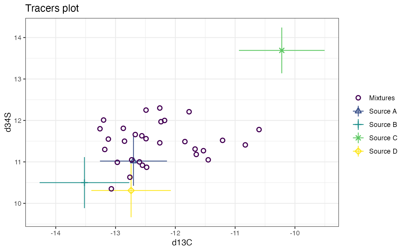
Plot the simmr_input data created from simmr_load

This function creates iso-space (AKA tracer-space or delta-space) plots. They are vital in determining whether the data are suitable for running in a SIMM.

# S3 method for simmr_input
plot(
  x,
  tracers = c(1, 2),
  title = "Tracers plot",
  xlab = colnames(x$mixtures)[tracers[1]],
  ylab = colnames(x$mixtures)[tracers[2]],
  sigmas = 1,
  group = 1:x$n_groups,
  mix_name = "Mixtures",
  ggargs = NULL,
  colour = TRUE,
  ...
)

Arguments

x: An object of class simmr_input created via the function simmr_load
tracers: The choice of tracers to plot. If there are more than two tracers, it is recommended to plot every pair of tracers to determine whether the mixtures lie in the mixing polygon defined by the sources
title: A title for the graph
xlab: The x-axis label. By default this is assumed to be delta-13C but can be made richer if required. See examples below.
ylab: The y-axis label. By default this is assumed to be delta-15N in per mil but can be changed as with the x-axis label
sigmas: The number of standard deviations to plot on the source values. Defaults to 1.
group: Which groups to plot. Can be a single group or multiple groups
mix_name: A optional string containing the name of the mixture objects, e.g. Geese.
ggargs: Extra arguments to be included in the ggplot (e.g. axis limits)
colour: If TRUE (default) creates a plot. If not, puts the plot in black and white
...: Not used

Value

isospace plot

Details

It is desirable to have the vast majority of the mixture observations to be inside the convex hull defined by the food sources. When there are more than two tracers (as in one of the examples below) it is recommended to plot all the different pairs of the food sources. See the vignette for further details of richer plots.

Author

Andrew Parnell <andrew.parnell@mu.ie>

Examples


# A simple example with 10 observations, 4 food sources and 2 tracers
data(geese_data_day1)
simmr_1 <- with(
  geese_data_day1,
  simmr_load(
    mixtures = mixtures,
    source_names = source_names,
    source_means = source_means,
    source_sds = source_sds,
    correction_means = correction_means,
    correction_sds = correction_sds,
    concentration_means = concentration_means
  )
)

# Plot
plot(simmr_1)


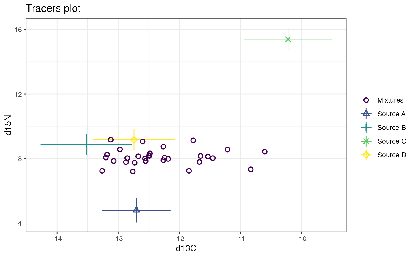
### A more complicated example with 30 obs, 3 tracers and 4 sources
data(simmr_data_2)
simmr_3 <- with(
  simmr_data_2,
  simmr_load(
    mixtures = mixtures,
    source_names = source_names,
    source_means = source_means,
    source_sds = source_sds,
    correction_means = correction_means,
    correction_sds = correction_sds,
    concentration_means = concentration_means
  )
)

# Plot 3 times - first default d13C vs d15N
plot(simmr_3)

# Now plot d15N vs d34S
plot(simmr_3, tracers = c(2, 3))

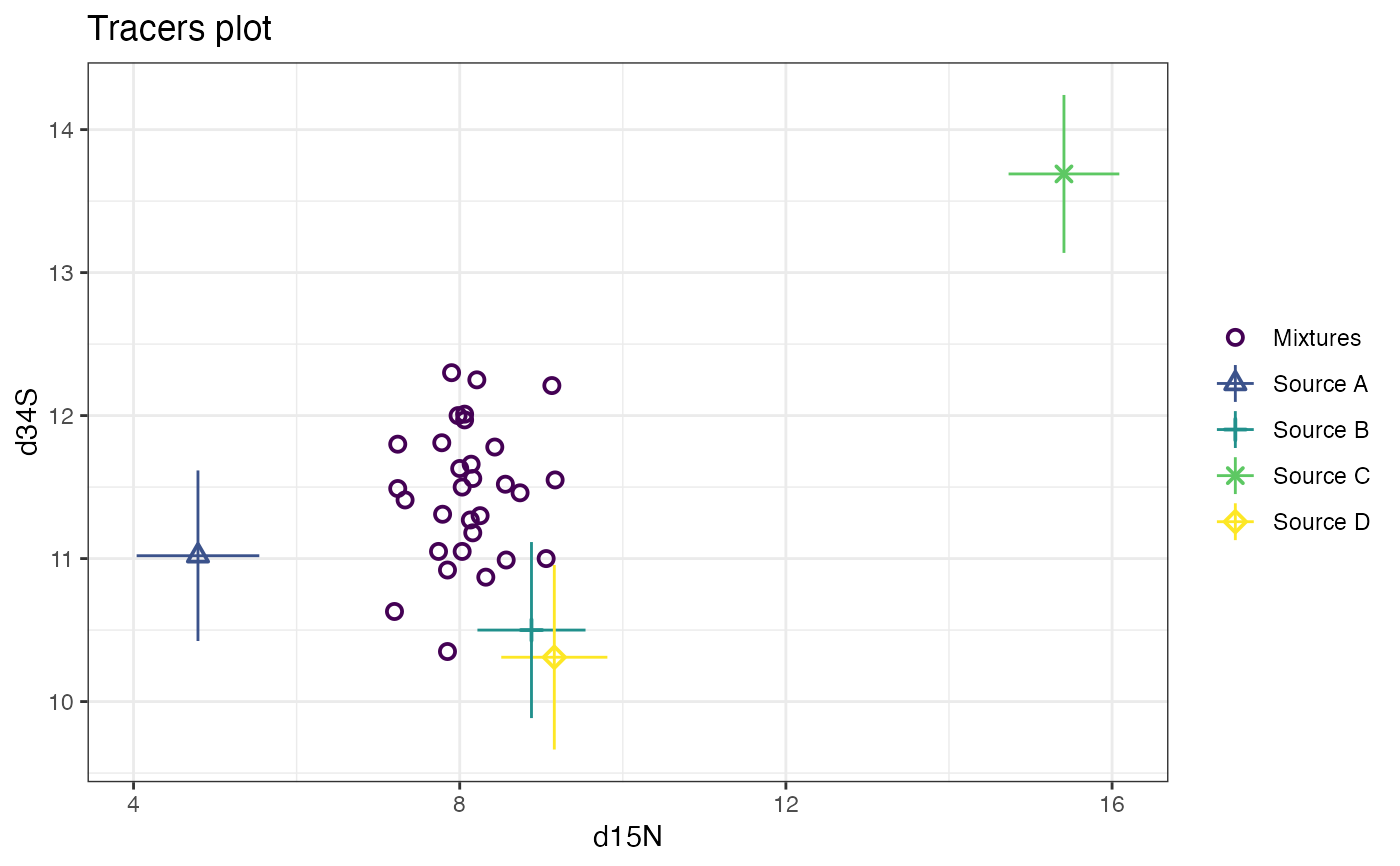# and finally d13C vs d34S
plot(simmr_3, tracers = c(1, 3))

# See vignette('simmr') for fancier x-axis labels

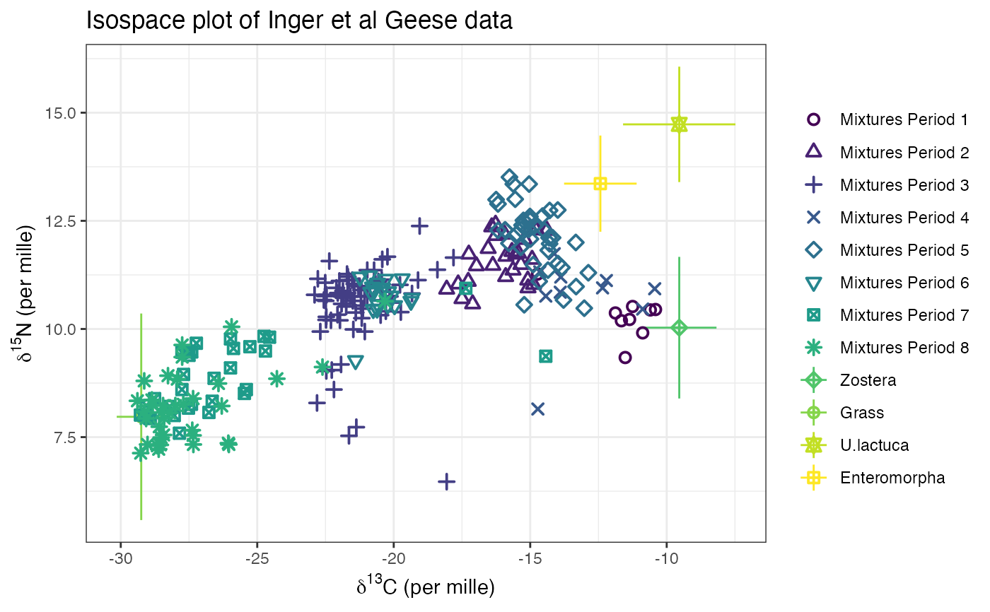
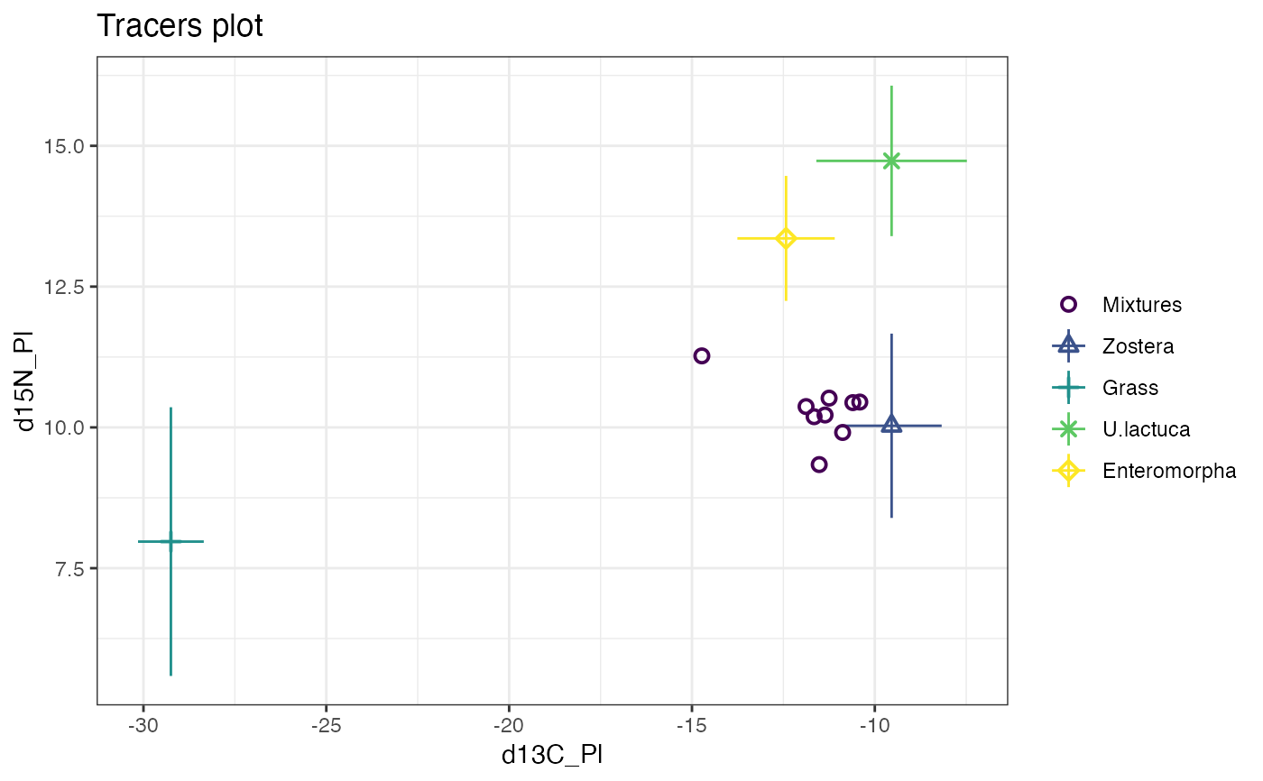
# An example with multiple groups - the Geese data from Inger et al 2006
data(geese_data)
simmr_4 <- with(
  geese_data,
  simmr_load(
    mixtures = mixtures,
    source_names = source_names,
    source_means = source_means,
    source_sds = source_sds,
    correction_means = correction_means,
    correction_sds = correction_sds,
    concentration_means = concentration_means,
    group = groups
  )
)

# Print
simmr_4
#> This is a valid simmr input object with 
#> 251  observations, 
#> 2 tracers, and 
#> 4 sources.
#> There are 8 groups.
#> The source names are: 
#> [1] "Zostera"      "Grass"        "U.lactuca"    "Enteromorpha"
#> .
#> The tracer names are: 
#> [1] "d13C_Pl" "d15N_Pl"
#> 
#> 

# Plot
plot(simmr_4,
  xlab = expression(paste(delta^13, "C (per mille)", sep = "")),
  ylab = expression(paste(delta^15, "N (per mille)", sep = "")),
  title = "Isospace plot of Inger et al Geese data"
) #'

Plot the `simmr_input` data created from `simmr_load`

Arguments

Value

Details

See also

Author

Examples