Plot different features of an object created from simmr_mcmc
or simmr_ffvb.
Source: R/plot.simmr_output.R
plot.simmr_output.RdThis function allows for 4 different types of plots of the simmr output
created from simmr_mcmc or simmr_ffvb. The
types are: histogram, kernel density plot, matrix plot (most useful) and
boxplot. There are some minor customisation options.
Arguments
- x
An object of class
simmr_outputcreated viasimmr_mcmcorsimmr_ffvb.- type
The type of plot required. Can be one or more of 'histogram', 'density', 'matrix', or 'boxplot'
- group
Which group(s) to plot.
- binwidth
The width of the bins for the histogram. Defaults to 0.05
- alpha
The degree of transparency of the plots. Not relevant for matrix plots
- title
The title of the plot.
- ggargs
Extra arguments to be included in the ggplot (e.g. axis limits)
- ...
Currently not used
Value
one or more of 'histogram', 'density', 'matrix', or 'boxplot'
Details
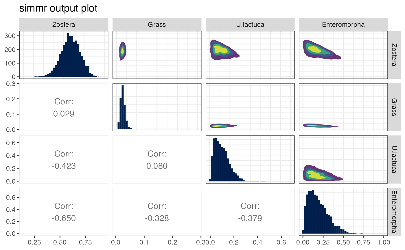
The matrix plot should form a necessary part of any SIMM analysis since it allows the user to judge which sources are identifiable by the model. Further detail about these plots is provided in the vignette. Some code from https://stackoverflow.com/questions/14711550/is-there-a-way-to-change-the-color-palette-for-ggallyggpairs-using-ggplot accessed March 2023
See also
See simmr_mcmc and simmr_ffvb for
creating objects suitable for this function, and many more examples. See
also simmr_load for creating simmr objects,
plot.simmr_input for creating isospace plots,
summary.simmr_output for summarising output.
Examples
# \donttest{
# A simple example with 10 observations, 2 tracers and 4 sources
# The data
data(geese_data)
# Load into simmr
simmr_1 <- with(
geese_data_day1,
simmr_load(
mixtures = mixtures,
source_names = source_names,
source_means = source_means,
source_sds = source_sds,
correction_means = correction_means,
correction_sds = correction_sds,
concentration_means = concentration_means
)
)
# Plot
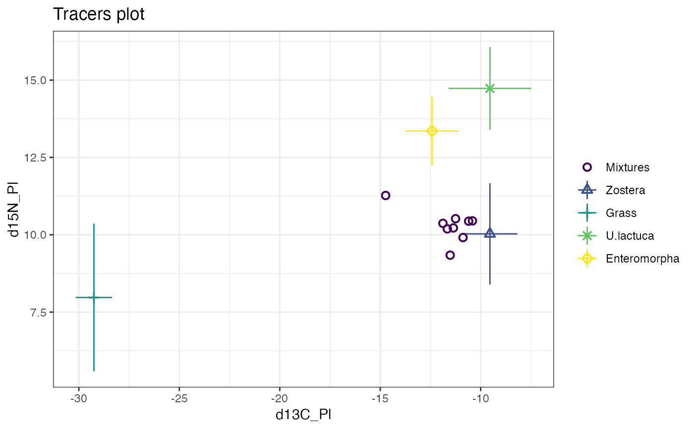
plot(simmr_1)
 # MCMC run
simmr_1_out <- simmr_mcmc(simmr_1)
#> Compiling model graph
#> Resolving undeclared variables
#> Allocating nodes
#> Graph information:
#> Observed stochastic nodes: 18
#> Unobserved stochastic nodes: 6
#> Total graph size: 136
#>
#> Initializing model
#>
# Plot
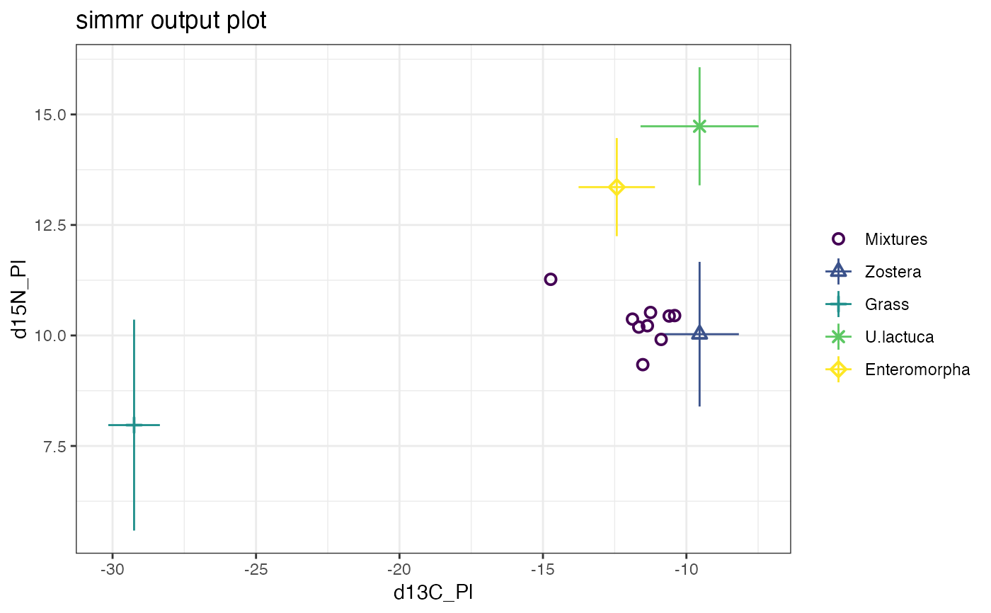
plot(simmr_1_out) # Creates all 4 plots
# MCMC run
simmr_1_out <- simmr_mcmc(simmr_1)
#> Compiling model graph
#> Resolving undeclared variables
#> Allocating nodes
#> Graph information:
#> Observed stochastic nodes: 18
#> Unobserved stochastic nodes: 6
#> Total graph size: 136
#>
#> Initializing model
#>
# Plot
plot(simmr_1_out) # Creates all 4 plots


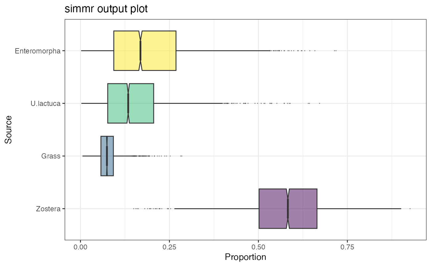
 plot(simmr_1_out, type = "boxplot")
 plot(simmr_1_out, type = "histogram")
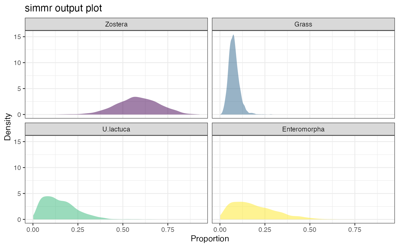
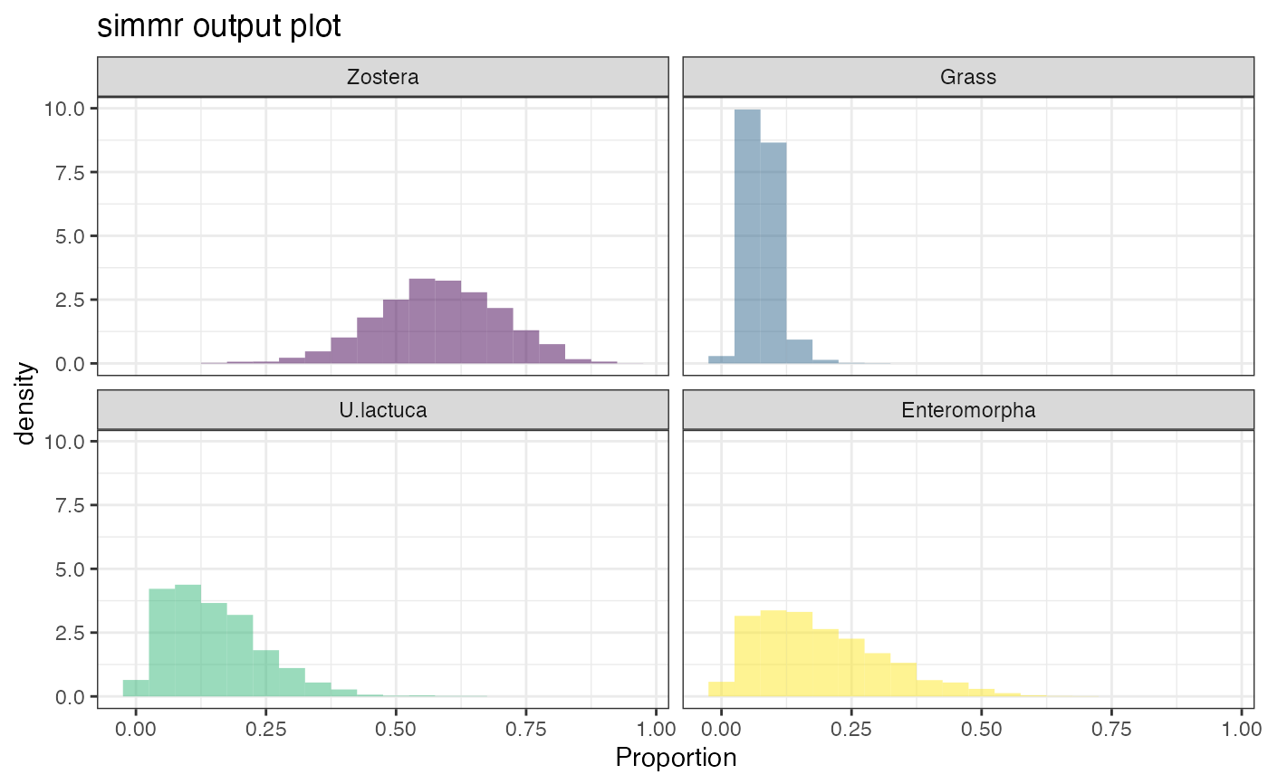 plot(simmr_1_out, type = "density")
 plot(simmr_1_out, type = "matrix")
 # }
# }