Summarises the output created with simmr_mcmc or simmr_ffvb

Produces textual summaries and convergence diagnostics for an object created with simmr_mcmc or simmr_ffvb. The different options are: 'diagnostics' which produces Brooks-Gelman-Rubin diagnostics to assess MCMC convergence, 'quantiles' which produces credible intervals for the parameters, 'statistics' which produces means and standard deviations, and 'correlations' which produces correlations between the parameters.

# S3 method for simmr_output
summary(
  object,
  type = c("diagnostics", "quantiles", "statistics", "correlations"),
  group = 1,
  ...
)

Arguments

object

An object of class simmr_output produced by the function simmr_mcmc or simmr_ffvb

type

The type of output required. At least none of 'diagnostics', 'quantiles', 'statistics', or 'correlations'.

group

Which group or groups the output is required for.

...

Not used

Value

A list containing the following components:

gelman

The convergence diagnostics

quantiles

The quantiles of each parameter from the posterior distribution

statistics

The means and standard deviations of each parameter

correlations

The posterior correlations between the parameters

Note that this object is reported silently so will be discarded unless the function is called with an object as in the example below.

Details

The quantile output allows easy calculation of 95 per cent credible intervals of the posterior dietary proportions. The correlations, along with the matrix plot in plot.simmr_output allow the user to judge which sources are non-identifiable. The Gelman diagnostic values should be close to 1 to ensure satisfactory convergence.

When multiple groups are included, the output automatically includes the results for all groups.

See also

See simmr_mcmc and simmr_ffvbfor creating objects suitable for this function, and many more examples. See also simmr_load for creating simmr objects, plot.simmr_input for creating isospace plots, plot.simmr_output for plotting output.

Author

Andrew Parnell <andrew.parnell@mu.ie>, Emma Govan

Examples

# \donttest{
# A simple example with 10 observations, 2 tracers and 4 sources

# The data
data(geese_data_day1)
simmr_1 <- with(
  geese_data_day1,
  simmr_load(
    mixtures = mixtures,
    source_names = source_names,
    source_means = source_means,
    source_sds = source_sds,
    correction_means = correction_means,
    correction_sds = correction_sds,
    concentration_means = concentration_means
  )
)

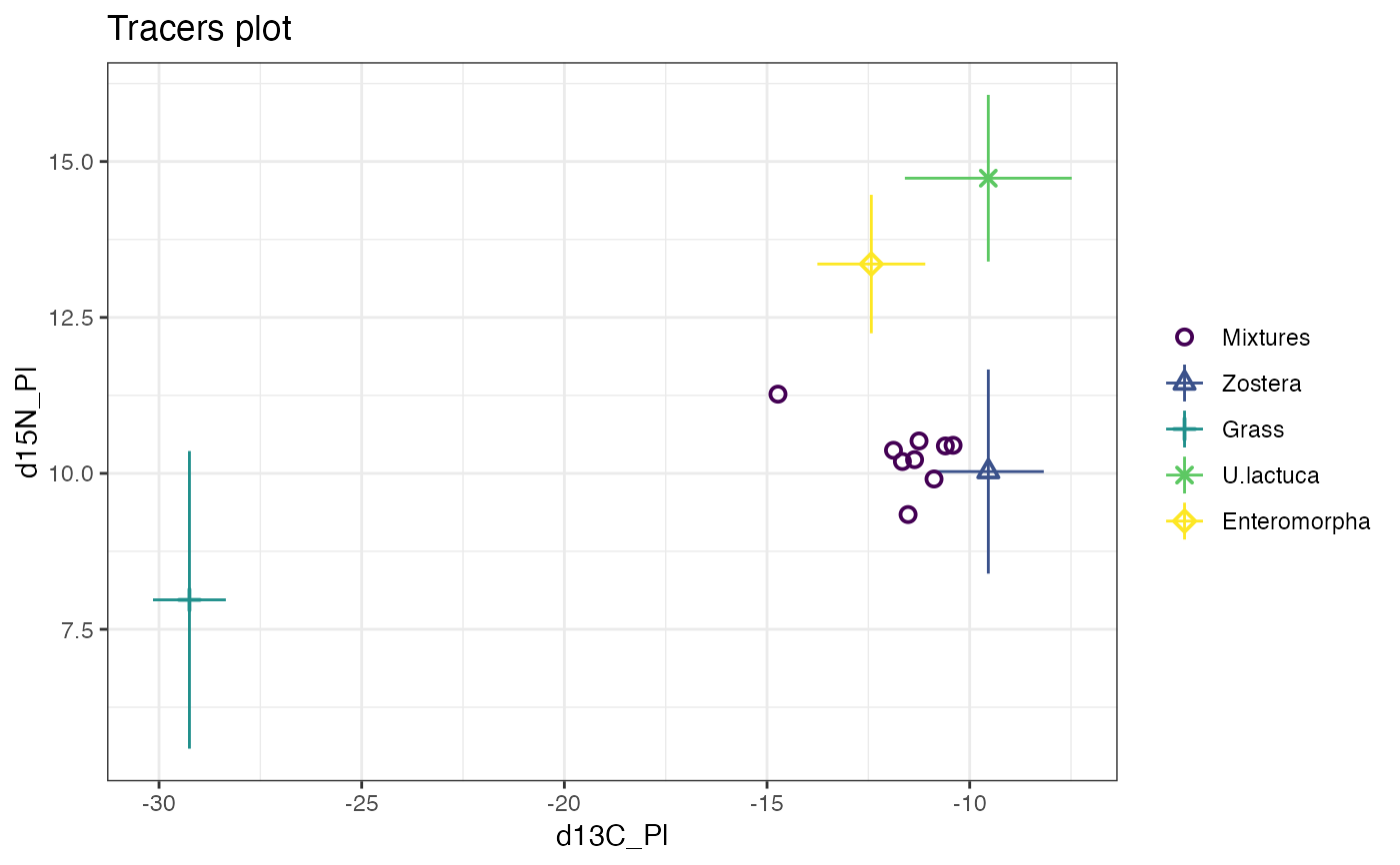
# Plot
plot(simmr_1)



# MCMC run
simmr_1_out <- simmr_mcmc(simmr_1)
#> Compiling model graph
#>    Resolving undeclared variables
#>    Allocating nodes
#> Graph information:
#>    Observed stochastic nodes: 18
#>    Unobserved stochastic nodes: 6
#>    Total graph size: 136
#> 
#> Initializing model
#> 

# Summarise
summary(simmr_1_out) # This outputs all the summaries
#> 
#> Summary for 1
#> R-hat values - these values should all be close to 1.
#> If not, try a longer run of simmr_mcmc.
#>     deviance      Zostera        Grass    U.lactuca Enteromorpha  sd[d13C_Pl] 
#>            1            1            1            1            1            1 
#>  sd[d15N_Pl] 
#>            1 
#>                2.5%    25%    50%    75%  97.5%
#> deviance     52.910 56.447 59.506 63.327 74.737
#> Zostera       0.333  0.505  0.583  0.665  0.807
#> Grass         0.028  0.058  0.074  0.092  0.137
#> U.lactuca     0.020  0.078  0.133  0.208  0.363
#> Enteromorpha  0.023  0.093  0.166  0.266  0.488
#> sd[d13C_Pl]   0.549  1.109  1.527  2.104  3.969
#> sd[d15N_Pl]   0.246  0.660  0.952  1.347  2.691
#>                mean    sd
#> deviance     60.552 5.645
#> Zostera       0.582 0.121
#> Grass         0.076 0.028
#> U.lactuca     0.150 0.094
#> Enteromorpha  0.192 0.126
#> sd[d13C_Pl]   1.717 0.909
#> sd[d15N_Pl]   1.085 0.642
#>              deviance Zostera  Grass U.lactuca Enteromorpha sd[d13C_Pl]
#> deviance        1.000  -0.273  0.133     0.164        0.111       0.673
#> Zostera        -0.273   1.000  0.037    -0.408       -0.666      -0.106
#> Grass           0.133   0.037  1.000     0.116       -0.342       0.246
#> U.lactuca       0.164  -0.408  0.116     1.000       -0.379       0.002
#> Enteromorpha    0.111  -0.666 -0.342    -0.379        1.000       0.046
#> sd[d13C_Pl]     0.673  -0.106  0.246     0.002        0.046       1.000
#> sd[d15N_Pl]     0.684  -0.196 -0.103     0.150        0.099       0.029
#>              sd[d15N_Pl]
#> deviance           0.684
#> Zostera           -0.196
#> Grass             -0.103
#> U.lactuca          0.150
#> Enteromorpha       0.099
#> sd[d13C_Pl]        0.029
#> sd[d15N_Pl]        1.000
summary(simmr_1_out, type = "diagnostics") # Just the diagnostics
#> 
#> Summary for 1
#> R-hat values - these values should all be close to 1.
#> If not, try a longer run of simmr_mcmc.
#>     deviance      Zostera        Grass    U.lactuca Enteromorpha  sd[d13C_Pl] 
#>            1            1            1            1            1            1 
#>  sd[d15N_Pl] 
#>            1 
# Store the output in an
ans <- summary(simmr_1_out,
  type = c("quantiles", "statistics")
)
#> 
#> Summary for 1
#>                2.5%    25%    50%    75%  97.5%
#> deviance     52.910 56.447 59.506 63.327 74.737
#> Zostera       0.333  0.505  0.583  0.665  0.807
#> Grass         0.028  0.058  0.074  0.092  0.137
#> U.lactuca     0.020  0.078  0.133  0.208  0.363
#> Enteromorpha  0.023  0.093  0.166  0.266  0.488
#> sd[d13C_Pl]   0.549  1.109  1.527  2.104  3.969
#> sd[d15N_Pl]   0.246  0.660  0.952  1.347  2.691
#>                mean    sd
#> deviance     60.552 5.645
#> Zostera       0.582 0.121
#> Grass         0.076 0.028
#> U.lactuca     0.150 0.094
#> Enteromorpha  0.192 0.126
#> sd[d13C_Pl]   1.717 0.909
#> sd[d15N_Pl]   1.085 0.642
# }