simmr: A package for fitting stable isotope mixing models via JAGS and FFVB in R

This package runs a simple Stable Isotope Mixing Model (SIMM) and is meant as a longer term replacement to the previous function SIAR.. These are used to infer dietary proportions of organisms consuming various food sources from observations on the stable isotope values taken from the organisms' tissue samples. However SIMMs can also be used in other scenarios, such as in sediment mixing or the composition of fatty acids. The main functions are simmr_load, simmr_mcmc, and simmr_ffvb. The help files contain examples of the use of this package. See also the vignette for a longer walkthrough.

Details

An even longer term replacement for properly running SIMMs is MixSIAR, which allows for more detailed random effects and the inclusion of covariates.

References

Andrew C. Parnell, Donald L. Phillips, Stuart Bearhop, Brice X. Semmens, Eric J. Ward, Jonathan W. Moore, Andrew L. Jackson, Jonathan Grey, David J. Kelly, and Richard Inger. Bayesian stable isotope mixing models. Environmetrics, 24(6):387–399, 2013.

Andrew C Parnell, Richard Inger, Stuart Bearhop, and Andrew L Jackson. Source partitioning using stable isotopes: coping with too much variation. PLoS ONE, 5(3):5, 2010.

Author

Andrew Parnell <andrew.parnell@mu.ie>

Examples

# \donttest{
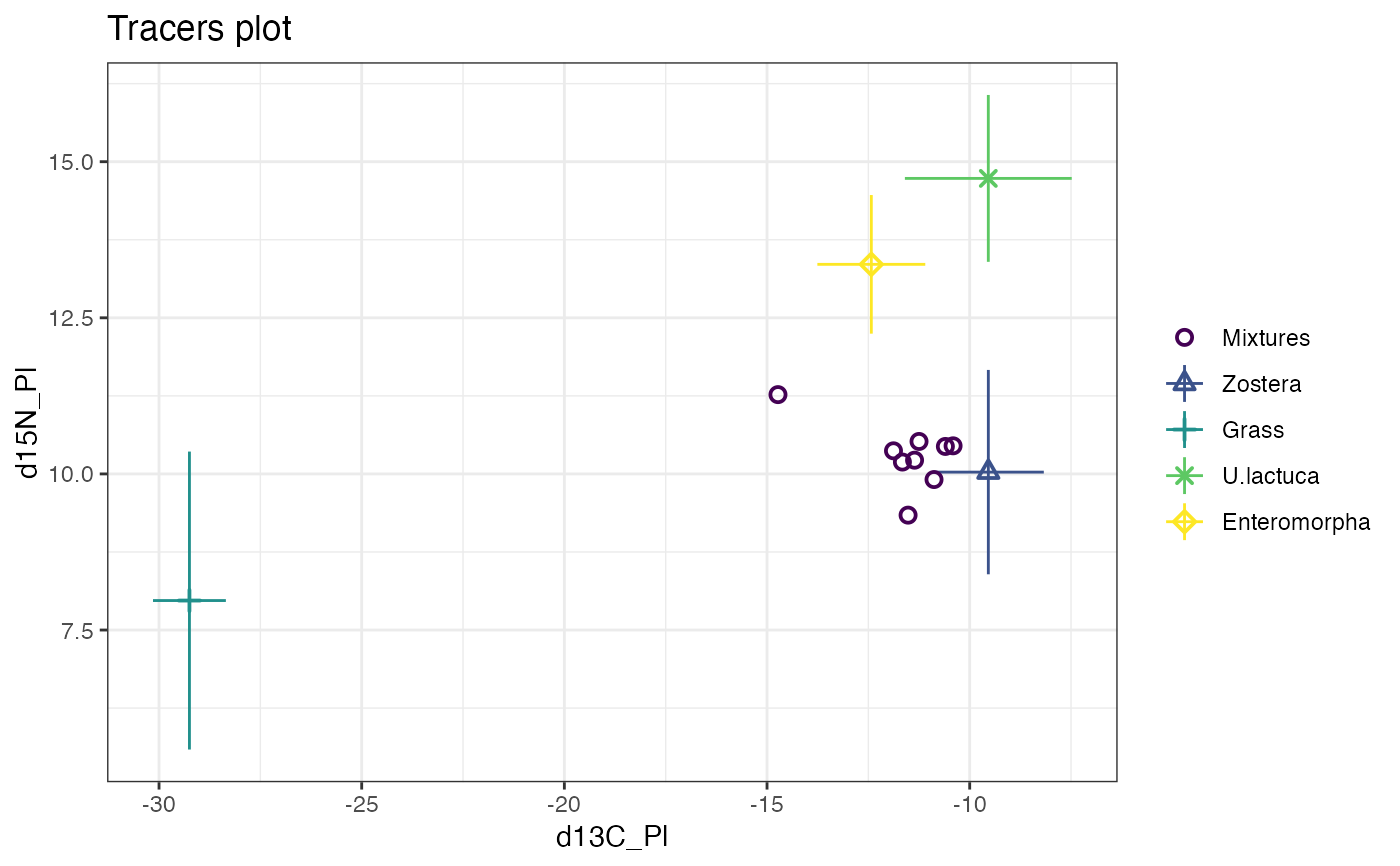
# A first example with 2 tracers (isotopes), 10 observations, and 4 food sources
data(geese_data_day1)
simmr_in <- with(
  geese_data_day1,
  simmr_load(
    mixtures = mixtures,
    source_names = source_names,
    source_means = source_means,
    source_sds = source_sds,
    correction_means = correction_means,
    correction_sds = correction_sds,
    concentration_means = concentration_means
  )
)

# Plot
plot(simmr_in)


# MCMC run
simmr_out <- simmr_mcmc(simmr_in)
#> Compiling model graph
#>    Resolving undeclared variables
#>    Allocating nodes
#> Graph information:
#>    Observed stochastic nodes: 18
#>    Unobserved stochastic nodes: 6
#>    Total graph size: 136
#> 
#> Initializing model
#> 

# Check convergence - values should all be close to 1
summary(simmr_out, type = "diagnostics")
#> 
#> Summary for 1
#> R-hat values - these values should all be close to 1.
#> If not, try a longer run of simmr_mcmc.
#>     deviance      Zostera        Grass    U.lactuca Enteromorpha  sd[d13C_Pl] 
#>            1            1            1            1            1            1 
#>  sd[d15N_Pl] 
#>            1 

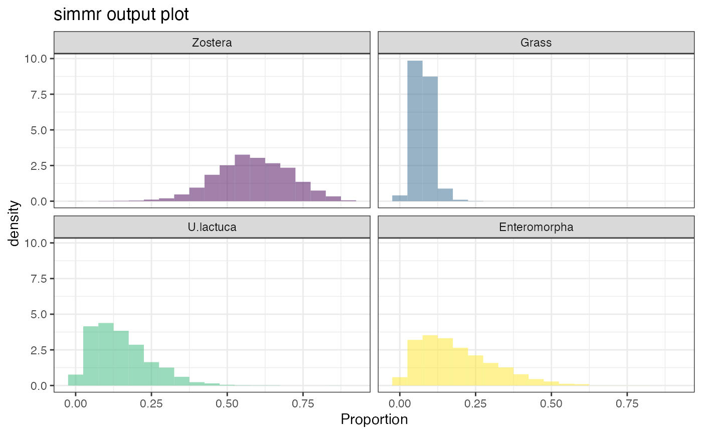
# Look at output
summary(simmr_out, type = "statistics")
#> 
#> Summary for 1
#>                mean    sd
#> deviance     60.573 5.503
#> Zostera       0.584 0.122
#> Grass         0.076 0.028
#> U.lactuca     0.150 0.097
#> Enteromorpha  0.189 0.123
#> sd[d13C_Pl]   1.697 0.894
#> sd[d15N_Pl]   1.097 0.646

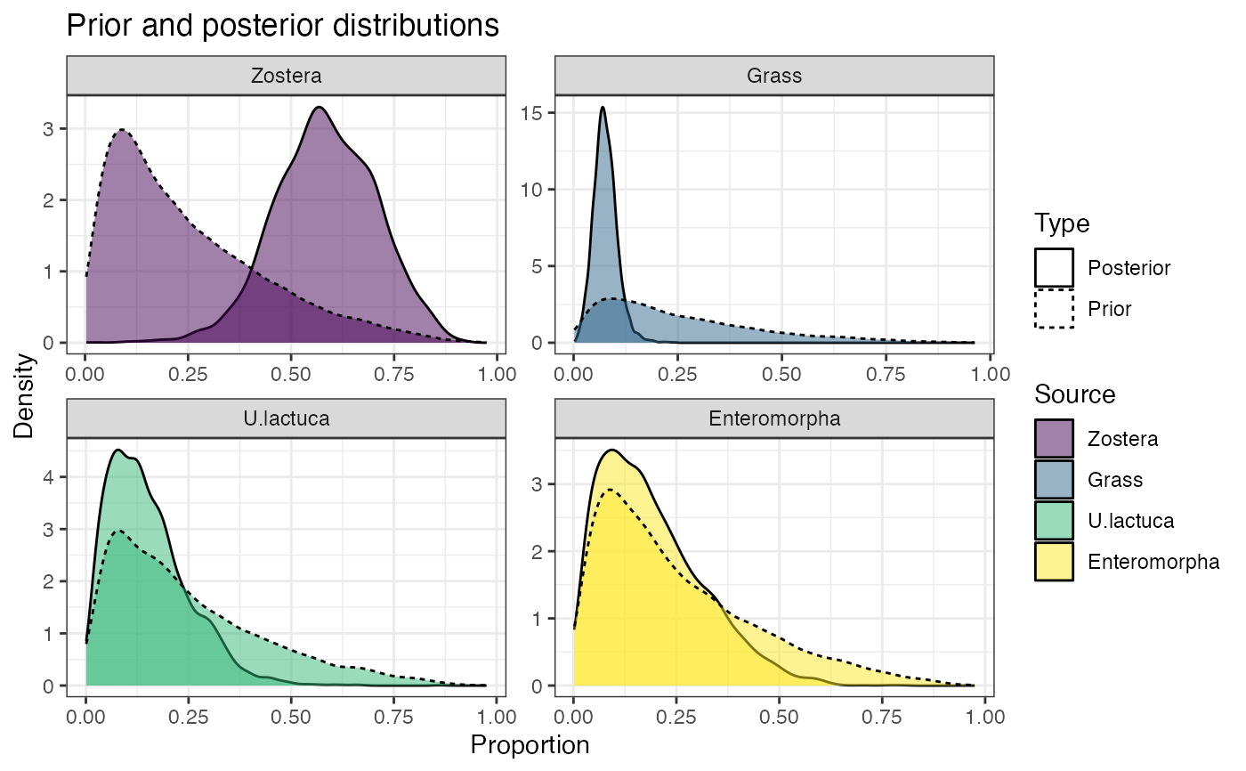
# Look at influence of priors
prior_viz(simmr_out)


# Plot output
plot(simmr_out, type = "histogram")

# }