Function to allow informative prior distribution to be included in simmr
Source:R/simmr_elicit.R
simmr_elicit.RdThe main simmr_mcmc function allows for a prior distribution
to be set for the dietary proportions. The prior distribution is specified
by transforming the dietary proportions using the centralised log ratio
(CLR). The simmr_elicit and simmr_elicit
functions allows the user to specify
prior means and standard deviations for each of the dietary proportions, and
then finds CLR-transformed values suitable for input into
simmr_mcmc.
Arguments
- n_sources
The number of sources required
- proportion_means
The desired prior proportion means. These should sum to 1. Should be a vector of length
n_sources- proportion_sds
The desired prior proportions standard deviations. These have no restricted sum but should be reasonable estimates for a proportion.
- n_sims
The number of simulations for which to run the optimisation routine.
Value
A list object with two components
- mean
The best estimates of the mean to use in
control.priorinsimmr_mcmc- sd
The best estimates of the standard deviations to use in
control.priorinsimmr_mcmc
Details
The function takes the desired proportion means and standard deviations,
and fits an optimised least squares to the means and standard deviations in
turn to produced CLR-transformed estimates for use in
simmr_mcmc. Using prior information in SIMMs is highly
desirable given the restricted nature of the inference. The prior
information might come from previous studies, other experiments, or other
observations of e.g. animal behaviour.
Due to the nature of the restricted space over which the dietary proportions
can span, and the fact that this function uses numerical optimisation, the
procedure will not match the target dietary proportion means and standard
deviations exactly. If this problem is severe, try increasing the
n_sims value.
Examples
# \donttest{
# Data set: 10 observations, 2 tracers, 4 sources
data(geese_data_day1)
simmr_1 <- with(
  geese_data_day1,
  simmr_load(
    mixtures = mixtures,
    source_names = source_names,
    source_means = source_means,
    source_sds = source_sds,
    correction_means = correction_means,
    correction_sds = correction_sds,
    concentration_means = concentration_means
  )
)

# MCMC run
simmr_1_out <- simmr_mcmc(simmr_1)
#> Compiling model graph
#>    Resolving undeclared variables
#>    Allocating nodes
#> Graph information:
#>    Observed stochastic nodes: 18
#>    Unobserved stochastic nodes: 6
#>    Total graph size: 136
#>
#> Initializing model
#>

# Look at the prior influence
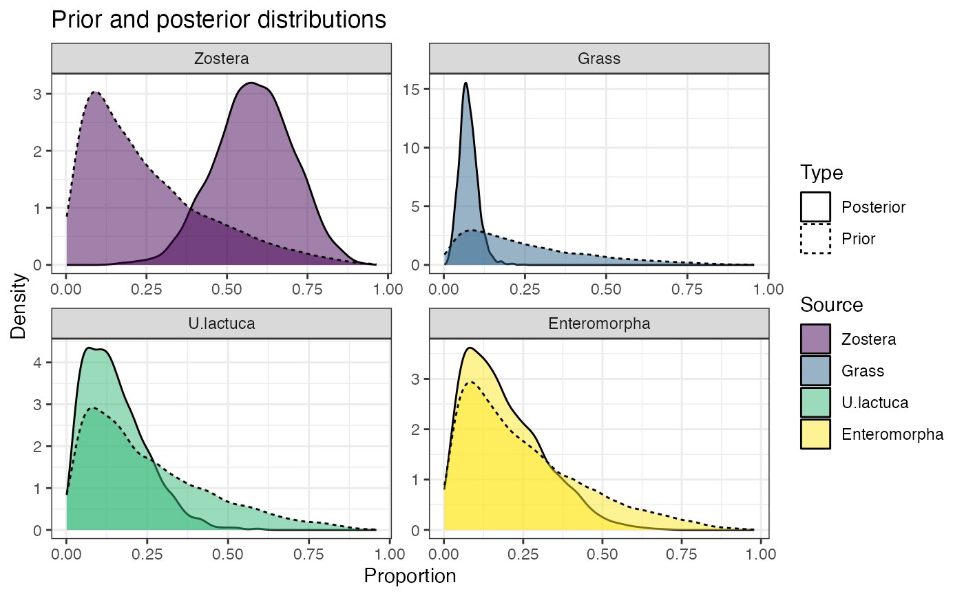
prior_viz(simmr_1_out)


# Summary
summary(simmr_1_out, "quantiles")
#>
#> Summary for 1
#>                2.5%    25%    50%    75%  97.5%
#> deviance     52.765 56.549 59.589 63.615 73.236
#> Zostera       0.339  0.505  0.585  0.667  0.809
#> Grass         0.028  0.057  0.073  0.093  0.140
#> U.lactuca     0.022  0.076  0.135  0.207  0.375
#> Enteromorpha  0.023  0.089  0.164  0.267  0.475
#> sd[d13C_Pl]   0.539  1.108  1.521  2.051  3.819
#> sd[d15N_Pl]   0.281  0.663  0.964  1.403  2.620
# A bit vague:
#           2.5%   25%   50%   75% 97.5%
# Source A 0.029 0.115 0.203 0.312 0.498
# Source B 0.146 0.232 0.284 0.338 0.453
# Source C 0.216 0.255 0.275 0.296 0.342
# Source D 0.032 0.123 0.205 0.299 0.465

# Now suppose I had prior information that:
# proportion means = 0.5,0.2,0.2,0.1
# proportion sds = 0.08,0.02,0.01,0.02
prior <- simmr_elicit(4, c(0.5, 0.2, 0.2, 0.1), c(0.08, 0.02, 0.01, 0.02))
#> Running elicitation optimisation routine...
#> Mean optimisation successful.
#> Standard deviation optimisation successful.
#> Best fit estimates provide proportion means of:
#> 0.5530.1880.1750.084
#>
#> ... and best fit standard deviations of:
#> 0.0540.0230.0210.021
#>
#> Check these match the input values before proceeding with a model run.

simmr_1a_out <- simmr_mcmc(simmr_1, prior_control =
list(means = prior$mean,
      sd = prior$sd,
      sigma_shape = c(3,3),
      sigma_rate = c(3/50, 3/50)))
#> Compiling model graph
#>    Resolving undeclared variables
#>    Allocating nodes
#> Graph information:
#>    Observed stochastic nodes: 18
#>    Unobserved stochastic nodes: 6
#>    Total graph size: 142
#>
#> Initializing model
#>

#' # Look at the prior influence now
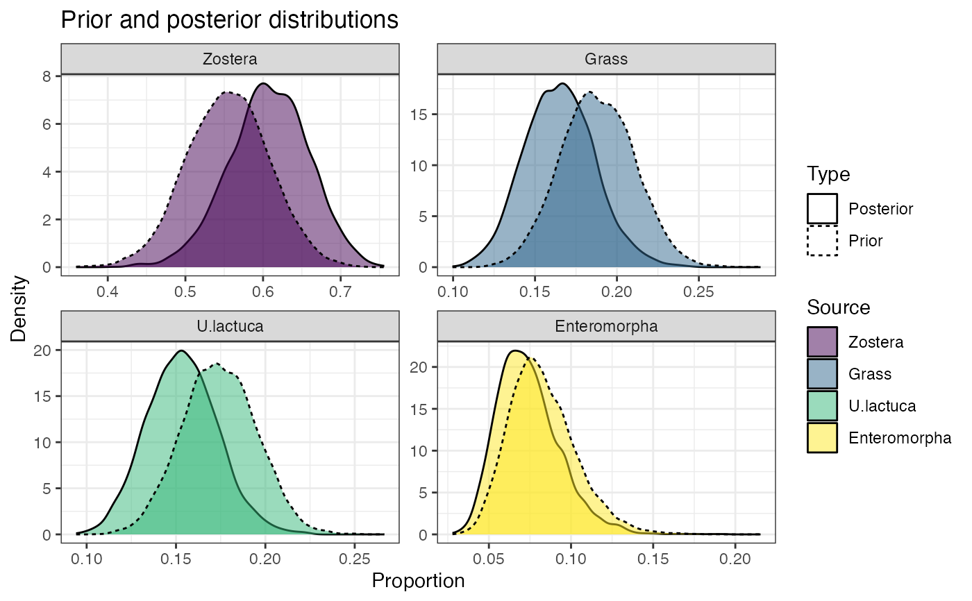
prior_viz(simmr_1a_out)


summary(simmr_1a_out, "quantiles")
#>
#> Summary for 1
#>                2.5%    25%    50%    75%  97.5%
#> deviance     59.410 64.665 67.591 71.284 79.645
#> Zostera       0.503  0.575  0.608  0.643  0.703
#> Grass         0.125  0.150  0.165  0.179  0.209
#> U.lactuca     0.116  0.140  0.153  0.167  0.194
#> Enteromorpha  0.044  0.061  0.072  0.085  0.118
#> sd[d13C_Pl]   1.229  2.199  2.873  3.780  6.372
#> sd[d15N_Pl]   0.247  0.601  0.859  1.204  2.324
# Much more precise:
#           2.5%   25%   50%   75% 97.5%
# Source A 0.441 0.494 0.523 0.553 0.610
# Source B 0.144 0.173 0.188 0.204 0.236
# Source C 0.160 0.183 0.196 0.207 0.228
# Source D 0.060 0.079 0.091 0.105 0.135
# }