Combine the dietary proportions from two food sources after running simmr
Source:R/combine_sources.R
combine_sources.RdThis function takes in an object of class simmr_output and combines
two of the food sources. It works for single and multiple group data.
combine_sources(
  simmr_out,
  to_combine = NULL,
  new_source_name = "combined_source"
)
Arguments
- simmr_out
An object of class
simmr_outputcreated fromsimmr_mcmcorsimmr_ffvb- to_combine
The names of exactly two sources. These should match the names given to
simmr_load.- new_source_name
A name to give to the new combined source.
Value
A new simmr_output object
Details
Often two sources either (1) lie in similar location on the iso-space plot,
or (2) are very similar in phylogenetic terms. In case (1) it is common to
experience high (negative) posterior correlations between the sources.
Combining them can reduce this correlation and improve precision of the
estimates. In case (2) we might wish to determine the joint amount eaten of
the two sources when combined. This function thus combines two sources after
a run of simmr_mcmc or simmr_ffvb (known as
a posteriori combination). The new object can then be called with
plot.simmr_input or plot.simmr_output to
produce iso-space plots of summaries of the output after combination.
See also
See simmr_mcmc and simmr_ffvb and
the associated vignette for examples.
Examples
# \donttest{
# The data
data(geese_data)
# Load into simmr
simmr_1 <- with(
geese_data_day1,
simmr_load(
mixtures = mixtures,
source_names = source_names,
source_means = source_means,
source_sds = source_sds,
correction_means = correction_means,
correction_sds = correction_sds,
concentration_means = concentration_means
)
)
# Plot
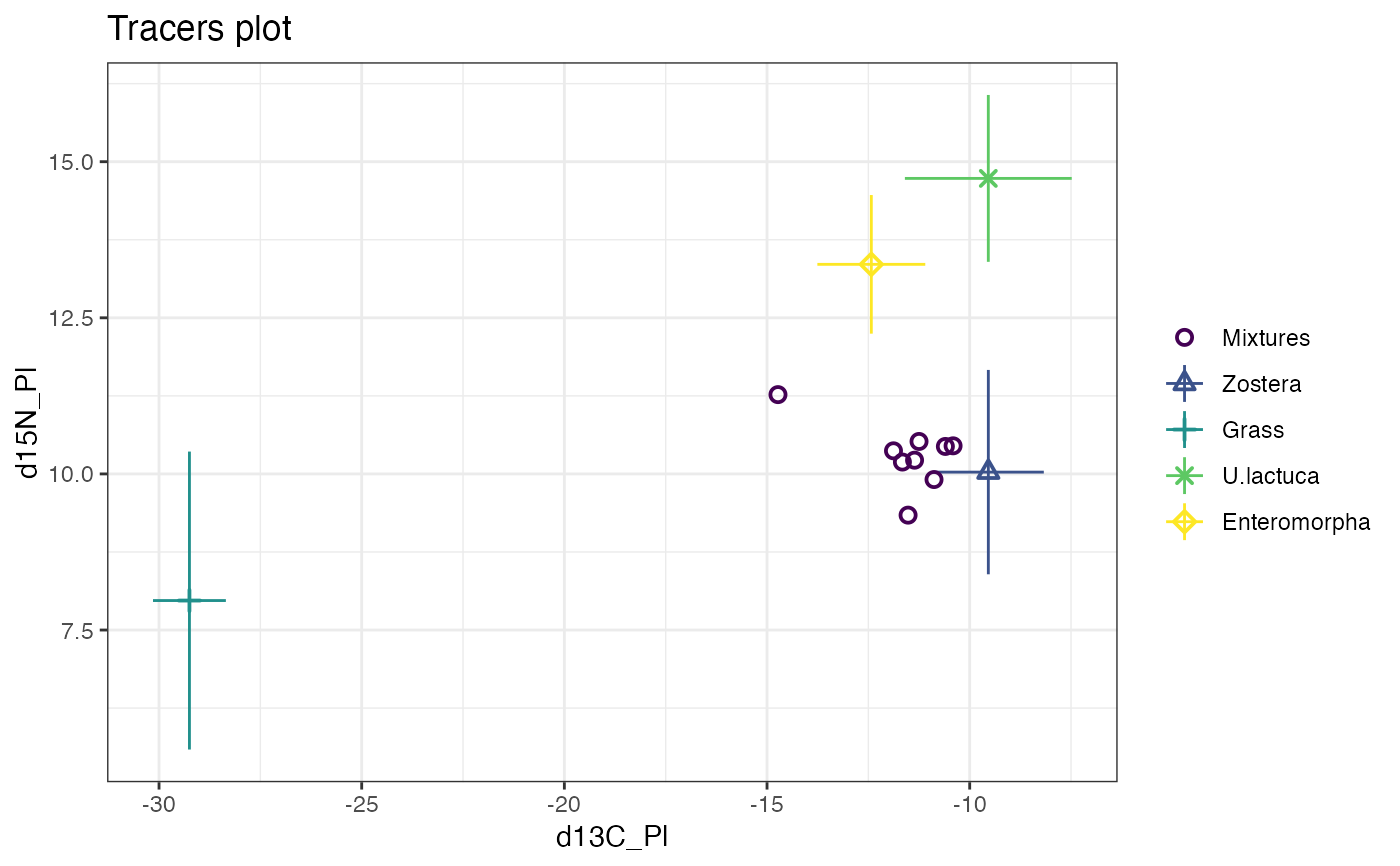
plot(simmr_1)
 # Print
simmr_1
#> This is a valid simmr input object with
#> 9 observations,
#> 2 tracers, and
#> 4 sources.
#> The source names are:
#> [1] "Zostera" "Grass" "U.lactuca" "Enteromorpha"
#> .
#> The tracer names are:
#> [1] "d13C_Pl" "d15N_Pl"
#>
#>
# MCMC run
simmr_1_out <- simmr_mcmc(simmr_1)
#> module glm loaded
#> Compiling model graph
#> Resolving undeclared variables
#> Allocating nodes
#> Graph information:
#> Observed stochastic nodes: 18
#> Unobserved stochastic nodes: 6
#> Total graph size: 136
#>
#> Initializing model
#>
# Print it
print(simmr_1_out)
#> This is a valid simmr input object with
#> 9 observations,
#> 2 tracers, and
#> 4 sources.
#> The source names are:
#> [1] "Zostera" "Grass" "U.lactuca" "Enteromorpha"
#> .
#> The tracer names are:
#> [1] "d13C_Pl" "d15N_Pl"
#>
#>
#> The input data has been run via simmr_mcmc and has produced
#> 3600 iterations over 4 MCMC chains.
#>
#>
# Summary
summary(simmr_1_out)
#>
#> Summary for 1
#> R-hat values - these values should all be close to 1.
#> If not, try a longer run of simmr_mcmc.
#> deviance Zostera Grass U.lactuca Enteromorpha sd[d13C_Pl]
#> 1 1 1 1 1 1
#> sd[d15N_Pl]
#> 1
#> 2.5% 25% 50% 75% 97.5%
#> deviance 52.844 56.474 59.529 63.273 73.518
#> Zostera 0.338 0.499 0.581 0.668 0.810
#> Grass 0.028 0.059 0.075 0.093 0.141
#> U.lactuca 0.021 0.075 0.134 0.204 0.366
#> Enteromorpha 0.021 0.091 0.170 0.269 0.487
#> sd[d13C_Pl] 0.533 1.128 1.546 2.104 3.865
#> sd[d15N_Pl] 0.262 0.640 0.939 1.349 2.622
#> mean sd
#> deviance 60.412 5.383
#> Zostera 0.581 0.121
#> Grass 0.077 0.028
#> U.lactuca 0.149 0.093
#> Enteromorpha 0.193 0.128
#> sd[d13C_Pl] 1.706 0.859
#> sd[d15N_Pl] 1.069 0.630
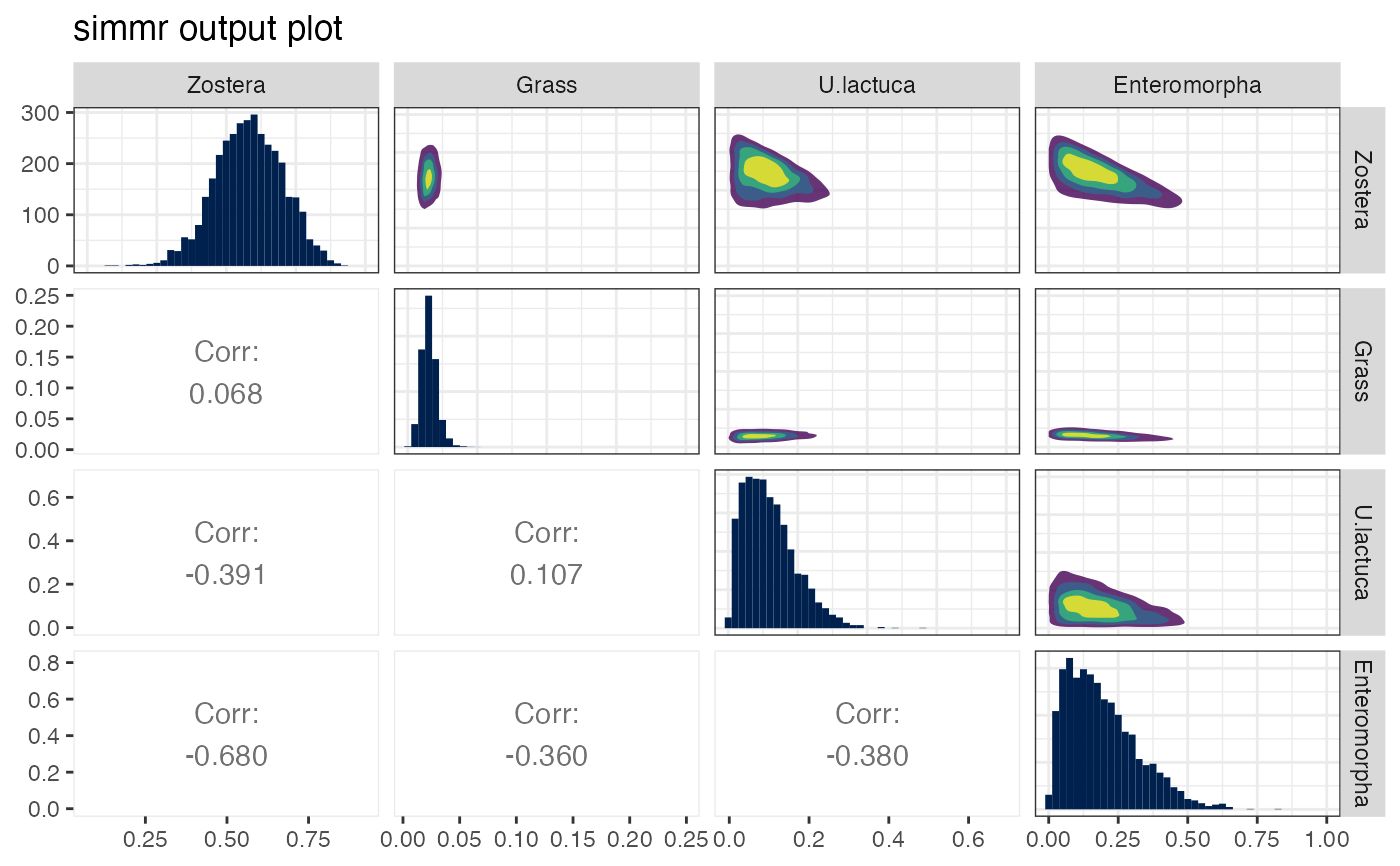
#> deviance Zostera Grass U.lactuca Enteromorpha sd[d13C_Pl]
#> deviance 1.000 -0.268 0.152 0.151 0.111 0.669
#> Zostera -0.268 1.000 0.068 -0.391 -0.680 -0.156
#> Grass 0.152 0.068 1.000 0.107 -0.360 0.270
#> U.lactuca 0.151 -0.391 0.107 1.000 -0.380 0.018
#> Enteromorpha 0.111 -0.680 -0.360 -0.380 1.000 0.076
#> sd[d13C_Pl] 0.669 -0.156 0.270 0.018 0.076 1.000
#> sd[d15N_Pl] 0.679 -0.153 -0.091 0.113 0.082 0.011
#> sd[d15N_Pl]
#> deviance 0.679
#> Zostera -0.153
#> Grass -0.091
#> U.lactuca 0.113
#> Enteromorpha 0.082
#> sd[d13C_Pl] 0.011
#> sd[d15N_Pl] 1.000
summary(simmr_1_out, type = "diagnostics")
#>
#> Summary for 1
#> R-hat values - these values should all be close to 1.
#> If not, try a longer run of simmr_mcmc.
#> deviance Zostera Grass U.lactuca Enteromorpha sd[d13C_Pl]
#> 1 1 1 1 1 1
#> sd[d15N_Pl]
#> 1
summary(simmr_1_out, type = "correlations")
#>
#> Summary for 1
#> deviance Zostera Grass U.lactuca Enteromorpha sd[d13C_Pl]
#> deviance 1.000 -0.268 0.152 0.151 0.111 0.669
#> Zostera -0.268 1.000 0.068 -0.391 -0.680 -0.156
#> Grass 0.152 0.068 1.000 0.107 -0.360 0.270
#> U.lactuca 0.151 -0.391 0.107 1.000 -0.380 0.018
#> Enteromorpha 0.111 -0.680 -0.360 -0.380 1.000 0.076
#> sd[d13C_Pl] 0.669 -0.156 0.270 0.018 0.076 1.000
#> sd[d15N_Pl] 0.679 -0.153 -0.091 0.113 0.082 0.011
#> sd[d15N_Pl]
#> deviance 0.679
#> Zostera -0.153
#> Grass -0.091
#> U.lactuca 0.113
#> Enteromorpha 0.082
#> sd[d13C_Pl] 0.011
#> sd[d15N_Pl] 1.000
summary(simmr_1_out, type = "statistics")
#>
#> Summary for 1
#> mean sd
#> deviance 60.412 5.383
#> Zostera 0.581 0.121
#> Grass 0.077 0.028
#> U.lactuca 0.149 0.093
#> Enteromorpha 0.193 0.128
#> sd[d13C_Pl] 1.706 0.859
#> sd[d15N_Pl] 1.069 0.630
ans <- summary(simmr_1_out, type = c("quantiles", "statistics"))
#>
#> Summary for 1
#> 2.5% 25% 50% 75% 97.5%
#> deviance 52.844 56.474 59.529 63.273 73.518
#> Zostera 0.338 0.499 0.581 0.668 0.810
#> Grass 0.028 0.059 0.075 0.093 0.141
#> U.lactuca 0.021 0.075 0.134 0.204 0.366
#> Enteromorpha 0.021 0.091 0.170 0.269 0.487
#> sd[d13C_Pl] 0.533 1.128 1.546 2.104 3.865
#> sd[d15N_Pl] 0.262 0.640 0.939 1.349 2.622
#> mean sd
#> deviance 60.412 5.383
#> Zostera 0.581 0.121
#> Grass 0.077 0.028
#> U.lactuca 0.149 0.093
#> Enteromorpha 0.193 0.128
#> sd[d13C_Pl] 1.706 0.859
#> sd[d15N_Pl] 1.069 0.630
# Plot
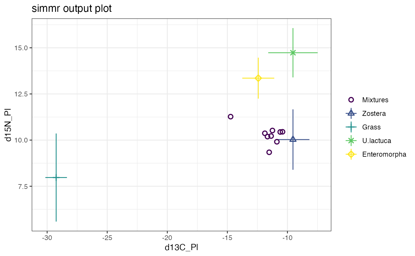
plot(simmr_1_out)
# Print
simmr_1
#> This is a valid simmr input object with
#> 9 observations,
#> 2 tracers, and
#> 4 sources.
#> The source names are:
#> [1] "Zostera" "Grass" "U.lactuca" "Enteromorpha"
#> .
#> The tracer names are:
#> [1] "d13C_Pl" "d15N_Pl"
#>
#>
# MCMC run
simmr_1_out <- simmr_mcmc(simmr_1)
#> module glm loaded
#> Compiling model graph
#> Resolving undeclared variables
#> Allocating nodes
#> Graph information:
#> Observed stochastic nodes: 18
#> Unobserved stochastic nodes: 6
#> Total graph size: 136
#>
#> Initializing model
#>
# Print it
print(simmr_1_out)
#> This is a valid simmr input object with
#> 9 observations,
#> 2 tracers, and
#> 4 sources.
#> The source names are:
#> [1] "Zostera" "Grass" "U.lactuca" "Enteromorpha"
#> .
#> The tracer names are:
#> [1] "d13C_Pl" "d15N_Pl"
#>
#>
#> The input data has been run via simmr_mcmc and has produced
#> 3600 iterations over 4 MCMC chains.
#>
#>
# Summary
summary(simmr_1_out)
#>
#> Summary for 1
#> R-hat values - these values should all be close to 1.
#> If not, try a longer run of simmr_mcmc.
#> deviance Zostera Grass U.lactuca Enteromorpha sd[d13C_Pl]
#> 1 1 1 1 1 1
#> sd[d15N_Pl]
#> 1
#> 2.5% 25% 50% 75% 97.5%
#> deviance 52.844 56.474 59.529 63.273 73.518
#> Zostera 0.338 0.499 0.581 0.668 0.810
#> Grass 0.028 0.059 0.075 0.093 0.141
#> U.lactuca 0.021 0.075 0.134 0.204 0.366
#> Enteromorpha 0.021 0.091 0.170 0.269 0.487
#> sd[d13C_Pl] 0.533 1.128 1.546 2.104 3.865
#> sd[d15N_Pl] 0.262 0.640 0.939 1.349 2.622
#> mean sd
#> deviance 60.412 5.383
#> Zostera 0.581 0.121
#> Grass 0.077 0.028
#> U.lactuca 0.149 0.093
#> Enteromorpha 0.193 0.128
#> sd[d13C_Pl] 1.706 0.859
#> sd[d15N_Pl] 1.069 0.630
#> deviance Zostera Grass U.lactuca Enteromorpha sd[d13C_Pl]
#> deviance 1.000 -0.268 0.152 0.151 0.111 0.669
#> Zostera -0.268 1.000 0.068 -0.391 -0.680 -0.156
#> Grass 0.152 0.068 1.000 0.107 -0.360 0.270
#> U.lactuca 0.151 -0.391 0.107 1.000 -0.380 0.018
#> Enteromorpha 0.111 -0.680 -0.360 -0.380 1.000 0.076
#> sd[d13C_Pl] 0.669 -0.156 0.270 0.018 0.076 1.000
#> sd[d15N_Pl] 0.679 -0.153 -0.091 0.113 0.082 0.011
#> sd[d15N_Pl]
#> deviance 0.679
#> Zostera -0.153
#> Grass -0.091
#> U.lactuca 0.113
#> Enteromorpha 0.082
#> sd[d13C_Pl] 0.011
#> sd[d15N_Pl] 1.000
summary(simmr_1_out, type = "diagnostics")
#>
#> Summary for 1
#> R-hat values - these values should all be close to 1.
#> If not, try a longer run of simmr_mcmc.
#> deviance Zostera Grass U.lactuca Enteromorpha sd[d13C_Pl]
#> 1 1 1 1 1 1
#> sd[d15N_Pl]
#> 1
summary(simmr_1_out, type = "correlations")
#>
#> Summary for 1
#> deviance Zostera Grass U.lactuca Enteromorpha sd[d13C_Pl]
#> deviance 1.000 -0.268 0.152 0.151 0.111 0.669
#> Zostera -0.268 1.000 0.068 -0.391 -0.680 -0.156
#> Grass 0.152 0.068 1.000 0.107 -0.360 0.270
#> U.lactuca 0.151 -0.391 0.107 1.000 -0.380 0.018
#> Enteromorpha 0.111 -0.680 -0.360 -0.380 1.000 0.076
#> sd[d13C_Pl] 0.669 -0.156 0.270 0.018 0.076 1.000
#> sd[d15N_Pl] 0.679 -0.153 -0.091 0.113 0.082 0.011
#> sd[d15N_Pl]
#> deviance 0.679
#> Zostera -0.153
#> Grass -0.091
#> U.lactuca 0.113
#> Enteromorpha 0.082
#> sd[d13C_Pl] 0.011
#> sd[d15N_Pl] 1.000
summary(simmr_1_out, type = "statistics")
#>
#> Summary for 1
#> mean sd
#> deviance 60.412 5.383
#> Zostera 0.581 0.121
#> Grass 0.077 0.028
#> U.lactuca 0.149 0.093
#> Enteromorpha 0.193 0.128
#> sd[d13C_Pl] 1.706 0.859
#> sd[d15N_Pl] 1.069 0.630
ans <- summary(simmr_1_out, type = c("quantiles", "statistics"))
#>
#> Summary for 1
#> 2.5% 25% 50% 75% 97.5%
#> deviance 52.844 56.474 59.529 63.273 73.518
#> Zostera 0.338 0.499 0.581 0.668 0.810
#> Grass 0.028 0.059 0.075 0.093 0.141
#> U.lactuca 0.021 0.075 0.134 0.204 0.366
#> Enteromorpha 0.021 0.091 0.170 0.269 0.487
#> sd[d13C_Pl] 0.533 1.128 1.546 2.104 3.865
#> sd[d15N_Pl] 0.262 0.640 0.939 1.349 2.622
#> mean sd
#> deviance 60.412 5.383
#> Zostera 0.581 0.121
#> Grass 0.077 0.028
#> U.lactuca 0.149 0.093
#> Enteromorpha 0.193 0.128
#> sd[d13C_Pl] 1.706 0.859
#> sd[d15N_Pl] 1.069 0.630
# Plot
plot(simmr_1_out)
 #> Registered S3 method overwritten by 'GGally':
#> method from
#> +.gg ggplot2
#> Registered S3 method overwritten by 'GGally':
#> method from
#> +.gg ggplot2
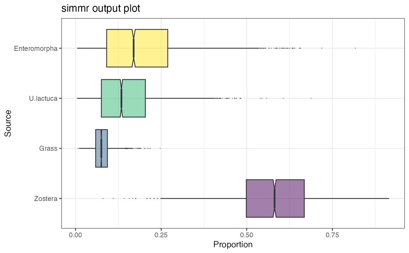
 plot(simmr_1_out, type = "boxplot")
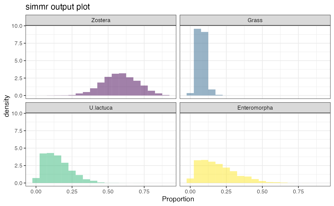
 plot(simmr_1_out, type = "histogram")
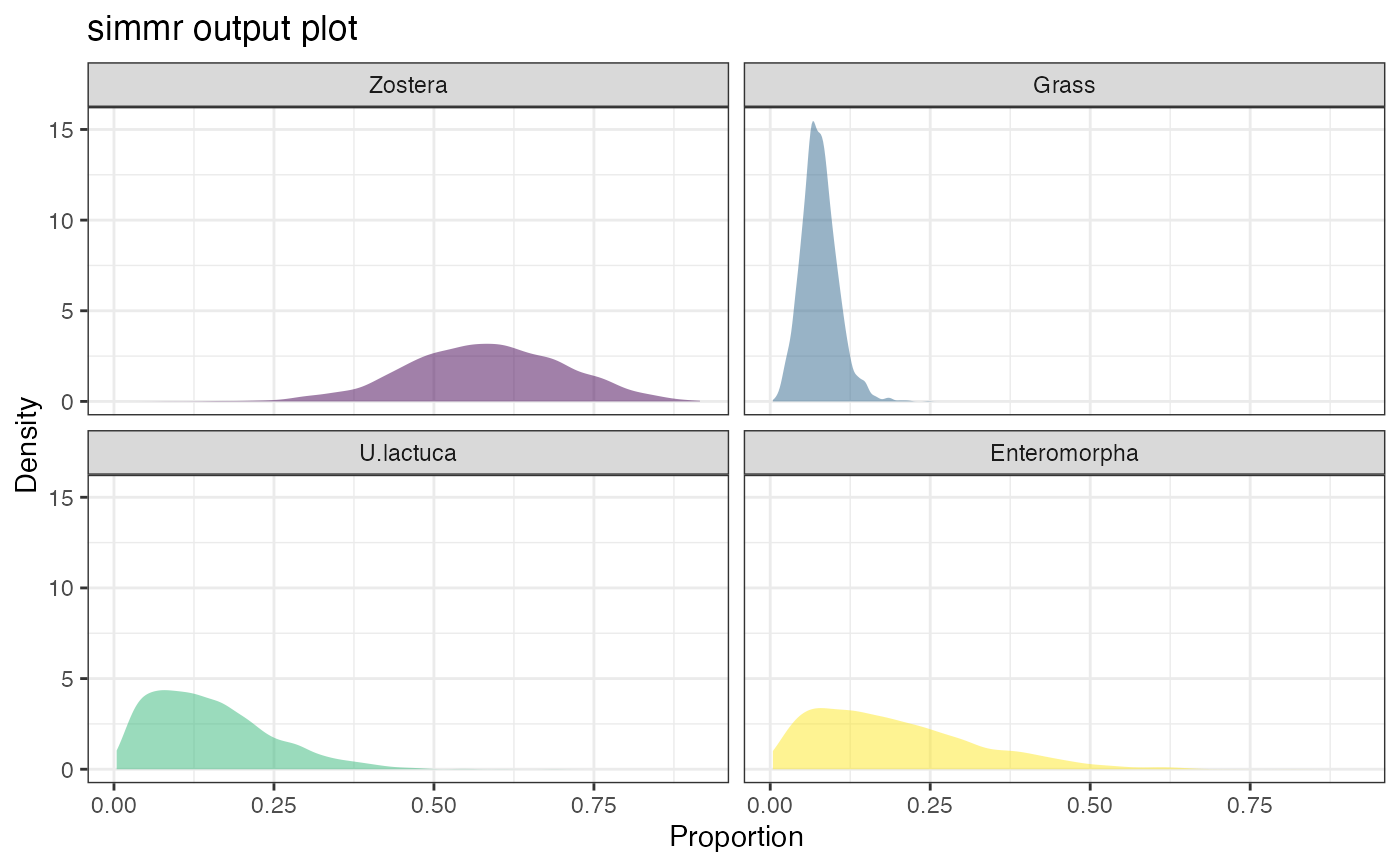
 plot(simmr_1_out, type = "density")
 plot(simmr_1_out, type = "matrix")
 simmr_out_combine <- combine_sources(simmr_1_out,
to_combine = c("U.lactuca", "Enteromorpha"),
new_source_name = "U.lac+Ent"
)
plot(simmr_out_combine$input)
simmr_out_combine <- combine_sources(simmr_1_out,
to_combine = c("U.lactuca", "Enteromorpha"),
new_source_name = "U.lac+Ent"
)
plot(simmr_out_combine$input)
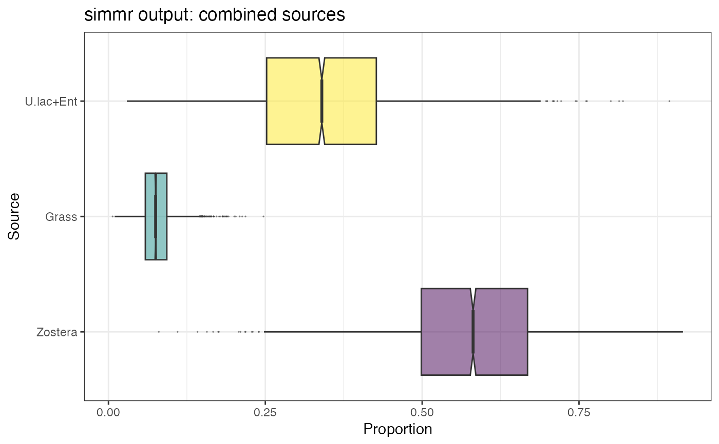
 plot(simmr_out_combine, type = "boxplot", title = "simmr output: combined sources")
 # }
# }